HOW TO GET LIVE CRICKET SCORE ON EXCEL SHEET ???

Hello friends I am  Neeraj Kumar, Welcome to the Independent learning- Excel Classes.

And today we are going to learn that how can we create an automated cricket scorecard in our Excel File. Please follow the below mentioned steps carefully to get it.

How get live cricket score on our excel sheet

1.  Firstly open your excel sheet and click Data tab like mention below screenshot.

2.    Click From Web Tab

3. Copy website URL Where do you take data from any cricket live score website.

     and pest open tap then press go.

     if you have receive any script error popup like mention screenshot press yes all time

4. Click yellow box.

5.  After click yellow box , box color change in green.

6. Click Import button

7. Select Range where you want get score.

8. After import data you get cricket score on your excel sheet.

9.  If you want score update automatic then press Data tab  then connection tab.like mention as              screenshot.

10. After open Dialog Box Click Properties tab

11. Click Refresh Every and fill minute As you wish.  

Thank you for your time. I hope it will help you to learn Excel tricks. Stay tuned for more cool excel tricks. Click here to watch excel training videos. Share if you have liked it.

You can submit your queries us at info.indelearning@gmail.com

                                   ----:The End:----

Read more »

Conditional Formatting 101

How to use CountA function In Conditional Formatting.

Hi friends please go through the you tube video for the full session. it is quick and easy.

in this video you will able to learn how to highlight certain cells using conditional formatting

Please don't forget to subscribe the YouTube channel.

Read more »

How to create a searchable drop-down in Excel in 5 minutes

Hi friends Welcome to independent learning, I am here with another great topic.

How to insert drop down list in excel

A Facebook friend were ask me to create the Searchable drop down menu in excel. So i have tried and hoping that this will help him.

In this article i will show you how to create a Searchable drop-down menu in excel. This Drop down will work like google search engine and you will be able to fetch data within a second from your resource directory.

I assume that your excel is compatible with macro and you have enabled the Developer Toolbar, and saved your file as .xlsm format. If you don't get this done, please do it first.

Setting Up things:

In Excel 2010 and 2013

Step 1- Click File Menu.
Step 2- Click Options.
Step 3- And in the Options dialog box, Click Customize Ribbon.
Step 4- Check the Developer box, then click the OK button.

In Excel 2007,

Step 1- Click Office button (Top most left, looks like windows logo)
Step 2- Click Excel Options.
Step 3- And in the Excel Options dialog box, Click Popular Tab.
Step 4- Check the Show Developer tab in the Ribbon box, then click the OK button.

Now you are all set for the preparation on Searchable Drop down list.

Watch the full practical video

Please follow the below mentioned steps carefully:

Step 1. Click Developer bar >> Click Insert >> In ActiveX Controls sector   select Combo Box to insert the same. See below:

Step 2. Draw the Combo box by Clicking and Dragging. Right Click the Combo box and then click on Properties.
Step 3. In Properties Dialog box please make following changes.
           (a) Select False in the AutoWordSelect field.
           (b) Specify a cell in the LinkedCell field. In this case, we enter G2.
           (c) Select 2-fmMatchEntryNone in the MatchEntry field.
           (d) Type DropDownList into the ListFillRange field then close.
See Below:

Step 4. Paste all your data in Column A.
Step 5. Paste this formula in the cell C2 =--ISNUMBER(IFERROR(SEARCH($g$2,A2,1),"")) and drag till last data cell In Column A. See Below:

Step 6. In Cell D2 Put this formula =IF(C2=1,COUNTIF($C$2:C2,1),"") and drag till last data cell In Column A. See below:

Step 7. In Cell E2 paste this                                                     formula =IFERROR(INDEX($A$2:$A$9,MATCH(ROWS($D$2:D2),$D$2:$D$9,0)),"") and drag till last data cell In Column A. See Below:

Step 8. Click On Formulas bar >> Click on Define Name >> Type "DropDownList" in the Name field.
Step 9. Put this =$E$2:INDEX($E$2:$E$9,MAX($D$2:$D$9),1) formula in Refers to box. Then Click Ok.  See Below:

Step 10. Dubble click the Combo Box that you inserted. VBA editor window will appear. Copy and paste the below mentioned code in the VBA editor.




Private Sub ComboBox1_GotFocus()

'Made by Vikash kumar

'The Independent Learning

'independentjournals.blogspot.com

'independentlearning.in

    ComboBox1.ListFillRange = "DropDownList"

    Me.ComboBox1.DropDown

End Sub




Step 11. Close the VBA editor, And deselect the Design mode. And your Searchable drop down list in excel is ready.

Please Download the practice file from here
Must watch the practice video. this will help you to understand the topic.

Please share this article if you like . Stay tunes for further videos
Feel free to reach us. Info.indelearning@gmail.com

Thanks in Advanced.
Happy Learning

Read more »

Hack your Excel ! Creating - Editing your own Custom list

Today's topic is creating a Custom List

Today we are going to discuss about custom lists, first you need to know that what is a Custom List in Excel? When ever we write Sunday or any day name and after we drags down, the Excel simply creates a list of days like Sunday, Monday, Tuesday etc. Its also happens when we write and drag a Month name. Like below mentioned video.

So how its happens ? All these questions are comes into our mind.

Q1. What is a Custom List ?

Q2. Can we create a Custom List of ours?

Q3. How to Edit an Custom List ?

Q4. How a Custom List works ?

You don't worry. all these questions will be answered in this article.

"see the video for full example and and practice session"

Follow the below mentioned steps carefully

Step 1 - Click on files tab in (Excel 2010). If you are using Excel 2007 then click on Office Button (right-top button).

Step 2 - Click on Options. Excel option window will appear.

Step 3 - Click on the Advanced tab. Left sixth from top. And drag till last. You will able t see Edit Custom list button as shown below image. Click Edit Custom Lists.

Step 4 - Write your entries by separating commas. (Sun, Moon, Earth, etc)

Step 5 - Click Add and Then Click OK.

Congratulations Your custom list has been added

Let's check it, Close Excel and open a saved file then write any of the words of the list and drag. Smile if working and do let me know if any error occurs.

Check now.

You can also delete any custom list my click Delete (Down to OK)

Happy Learning

Read more »

Hack your Excel: Unprotect Excel sheet without Password (No VBA, No Software)

Hack your Excel: Unprotect Excel sheet without Password 

Disclaimer: This tutorial is for educational purposes only and is not intended to be put into practise unless you have authorised access to the files you are trying to break into.

      Have you forgotten MS Excel sheet’s password and you are trying to get it done from google, trust me you will redirected to various websites. They suggest you to download their software, addins applications. But will not solve your purpose.

Try this trick

          Here is the way you which can help you for to crack your excel sheet password. This article will help you to Unprotect you protected sheet without password.

Please mind this with this trick you can only unprotect SHEETS not the WORKBOOKs.

Please do following necessary changes in your system as shown below:-

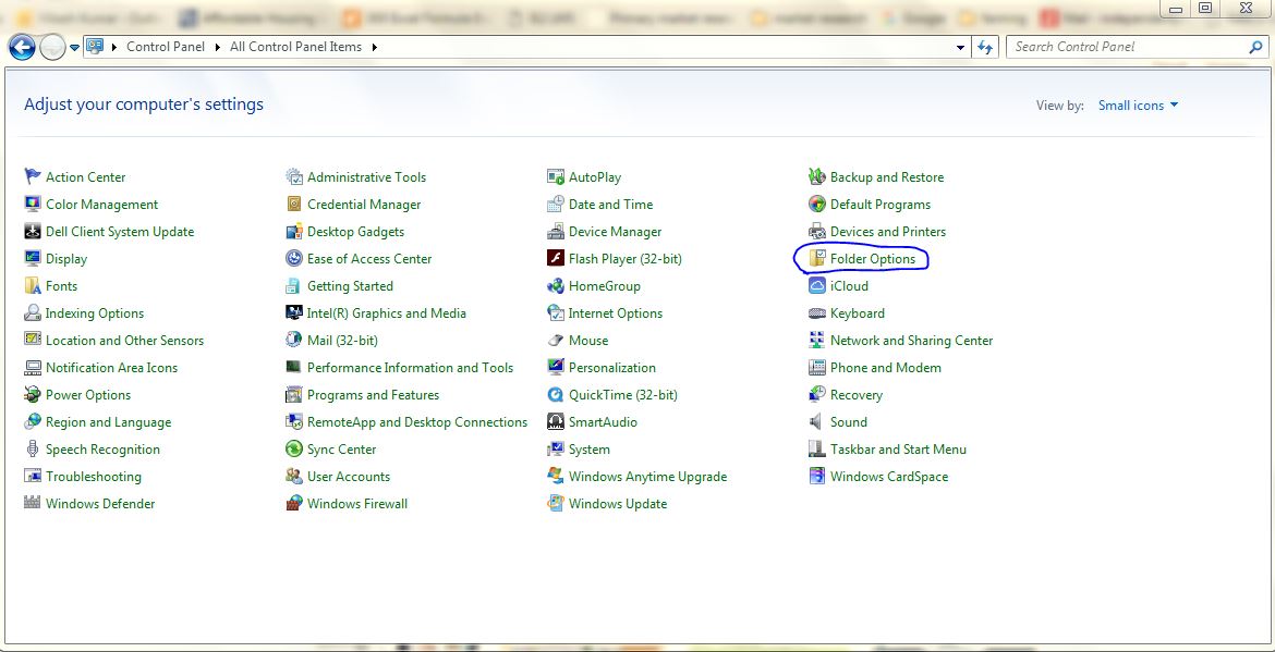
1. Open Control Panel and Select Folder Option

2. Menu bar click View  and Do uncheck the “Hide Extensions from known files types”. Click Aply and OK.

Now your system is ready for unprotect sheets without password.

Follow the steps shown below:

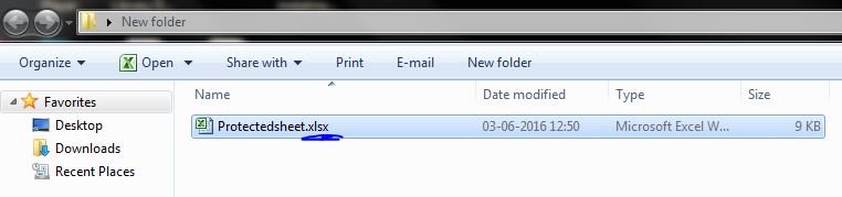
1. Select the Desired Excel File, change extension (Press F2) .zip.

2. Open zipped Folder

3. Open xl folder and forget about others.

4. In the xl folder you will get few more folders, open worksheets folder and forget about others.

5. In the worksheets folder you will able to see all your sheets with are already in your protected sheet.

6. Extract you protected sheet in a new folder(outside the current zipped folder).

7. Open file with Notepad or Right Click on file and select Edit option.

8. If you are using MS office version 2007/2010 then search  <sheetProtection password=****/> tag  and delete it.

9. If you are using MS office version 2013 then searc  < sheetProtection algorithmName=****/> tag  and delete it.

10. Save the file and Close. Replace new xml file with the original xml files witch are in the Zipped folder.

11. Close the zipped file.

12. Change the extension from .zip to .xlsx.

Enjoy you have unprotected the sheets successfully .

Click Here To contact us

Read more »